Regression with Hundred Hammers

In this notebook we will explain how to use the HundredHammers library to perfom a basic model selection and hyperparameter optimization for a classification problem.

To do this, we will use one of the example datasets available in the scikit-learn library.

import logging

import hundred_hammers as hh
from hundred_hammers.model_zoo import (
    DummyRegressor,
    Ridge,
    DecisionTreeRegressor,
    KNeighborsRegressor,
)

from sklearn.datasets import load_diabetes
from sklearn.metrics import mean_squared_error

First we store the data in the X (input) and y (target) variables.

data = load_diabetes()
X = data.data
y = data.target

We are going to first train some models with their default configuration. If you don’t specify the models that you want to use, some regression models will be chosen for you.

To see which models are chosen by default, you can check the DEFAULT_REGRESSION_MODELS variable

hh.model_zoo.DEFAULT_REGRESSION_MODELS

[('Dummy Mean', DummyRegressor(), {}),
 ('Dummy Median', DummyRegressor(strategy='median'), {}),
 ('Linear Regression', LinearRegression(), {}),
 ('Decision Tree', DecisionTreeRegressor(), {}),
 ('SVR', SVR(), {}),
 ('Linear SVR', LinearSVR(), {}),
 ('Ridge', Ridge(), {}),
 ('Passive Aggressive', PassiveAggressiveRegressor(), {}),
 ('KNN', KNeighborsRegressor(), {}),
 ('Neural Network Regressor', MLPRegressor(), {}),
 ('Gaussian Process', GaussianProcessRegressor(), {}),
 ('Random Forest', RandomForestRegressor(), {}),
 ('AdaBoost', AdaBoostRegressor(), {}),
 ('Gradient Boosting', GradientBoostingRegressor(), {})]

Notice that it is composed of a list of tuples. Each tuple contains the name we give to the regressors, an instance of the class that implements the regression model and a grid of hyperparameters (which now is empty, but will be explained later).

Those are the models that we are going to use now.

Evaluation with default models

First create the HundredHammersRegressor object

hh_models = hh.HundredHammersRegressor(show_progress_bar=True)

Then evaluate the models. Apart from the actual data (the variables X and y), you can pass other parameters. optim_hyper checks whether we want to optimize the hyperparameters of the models and n_grid_points controls how many values from each hyperparameter to check in the optimization.

Since we don’t want to optimize the hyperparameters, optim_hyper will stay as false.

# configure the logger
hh.hh_logger.setLevel(logging.WARNING)

# Evaluate the models and store the results in a variable
df_results = hh_models.evaluate(X, y, optim_hyper=False)

Evaluating models...: 100%|██████████| 14/14 [00:52<00:00,  3.77s/it]

Notice the line above the evaluation of the models. This configures the logger to only show warnings (of which there should be none). The setting you most likely would want to use in an interactive enviroment would be logging.INFO, since you get information about each model in “real time”.

If you want to see more detailed information, you can set the level to logging.DEBUG. It outputs a lot of information, but it might be useful if you encounter a bug.

For the purposes of this notebook, it will be kept to logging.WARNING but you are welcome to change it if you are running this notebook locally.

We can now show the results of our execution

df_results

	Model	Avg R2 (Validation Train)	Std R2 (Validation Train)	Avg R2 (Validation Test)	Std R2 (Validation Test)	Avg R2 (Train)	Std R2 (Train)	Avg R2 (Test)	Std R2 (Test)	Avg MSE (Validation Train)	...	Avg MSE (Test)	Std MSE (Test)	Avg MAE (Validation Train)	Std MAE (Validation Train)	Avg MAE (Validation Test)	Std MAE (Validation Test)	Avg MAE (Train)	Std MAE (Train)	Avg MAE (Test)	Std MAE (Test)
0	Dummy Mean	0.000000	0.000000	-0.023206	0.033628	0.000000	0.000000e+00	-0.001337	0.000000e+00	6125.118931	...	5134.783503	0.000000e+00	67.301695	1.188564	67.615074	3.943941	67.339534	1.421085e-14	59.227456	7.105427e-15
1	Dummy Median	-0.027476	0.007274	-0.050684	0.071611	-0.025922	0.000000e+00	-0.045202	0.000000e+00	6293.183322	...	5359.719101	9.094947e-13	66.517990	1.217067	66.993618	4.993507	66.566572	0.000000e+00	59.044944	0.000000e+00
2	Linear Regression	0.556522	0.015235	0.514558	0.067539	0.553925	0.000000e+00	0.332233	0.000000e+00	2715.353061	...	3424.259334	0.000000e+00	42.404995	0.829168	43.952508	3.145022	42.593344	0.000000e+00	46.173585	0.000000e+00
3	Decision Tree	1.000000	0.000000	-0.046363	0.200661	1.000000	0.000000e+00	-0.452581	7.741044e-02	0.000000	...	7448.729213	3.969551e+02	0.000000	0.000000	61.592362	5.524460	0.000000	0.000000e+00	72.787640	2.030020e+00
4	SVR	0.159545	0.009264	0.126855	0.062307	0.186951	2.775558e-17	0.128119	0.000000e+00	5147.222487	...	4470.939683	0.000000e+00	59.987041	1.025494	61.080993	4.554385	58.932403	0.000000e+00	53.268617	0.000000e+00
5	Linear SVR	-0.480290	0.021770	-0.499608	0.177843	-0.380897	2.104066e-03	-0.515761	2.670427e-03	9068.418326	...	7772.710116	1.369376e+01	72.936544	1.610525	73.117766	7.733969	71.098948	3.656171e-02	67.626756	6.017854e-02
6	Ridge	0.445599	0.013815	0.419461	0.046400	0.465084	0.000000e+00	0.340980	5.551115e-17	3394.642031	...	3379.406308	0.000000e+00	49.381703	0.756940	50.079365	3.114845	48.381085	7.105427e-15	46.566795	0.000000e+00
7	Passive Aggressive	0.506681	0.026801	0.471776	0.060789	0.517667	9.373723e-03	0.358801	5.003282e-03	3020.352370	...	3288.020684	2.565646e+01	45.207007	1.403516	46.656725	3.233495	44.703236	6.186625e-01	45.272923	2.780478e-01
8	KNN	0.615279	0.021038	0.410247	0.083013	0.618820	0.000000e+00	0.172488	0.000000e+00	2354.986676	...	4243.422022	0.000000e+00	37.785156	1.130082	46.627299	3.687450	37.339377	0.000000e+00	49.492135	0.000000e+00
9	Neural Network Regressor	-2.925185	0.119621	-2.988113	0.350351	-2.917495	9.059604e-02	-3.644418	1.081171e-01	24040.326288	...	23816.235196	5.544168e+02	134.976709	3.010464	135.014455	9.449213	134.932019	1.912264e+00	137.552821	1.910063e+00
10	Gaussian Process	0.995085	0.001516	-13.683252	6.935421	0.984183	1.110223e-16	-9.864145	0.000000e+00	30.042210	...	55710.543741	7.275958e-12	2.979676	0.408915	182.608347	32.059452	5.759758	0.000000e+00	144.352684	2.842171e-14
11	Random Forest	0.925400	0.003492	0.451311	0.081209	0.924440	1.996863e-03	0.261153	1.513057e-02	456.784823	...	3788.750941	7.758846e+01	17.203293	0.450834	46.492412	3.162357	17.225159	2.502492e-01	48.277247	5.898557e-01
12	AdaBoost	0.687707	0.017497	0.460084	0.072768	0.662306	5.843726e-03	0.279929	1.969705e-02	1911.433685	...	3692.470967	1.010051e+02	38.272124	1.042228	46.951305	3.079916	39.829220	4.565226e-01	47.444248	5.013379e-01
13	Gradient Boosting	0.889395	0.008559	0.441646	0.077073	0.857853	1.110223e-16	0.208258	1.787313e-03	677.065400	...	4059.994938	9.165209e+00	20.760164	0.796809	46.463974	3.126900	23.559587	3.552714e-15	49.229710	1.154214e-01

14 rows × 25 columns

That’s an ok way of displaying the result, but tables can sometimes be hard to read, this is why we also implement a couple of functions to display the information of the table in a more readable format.

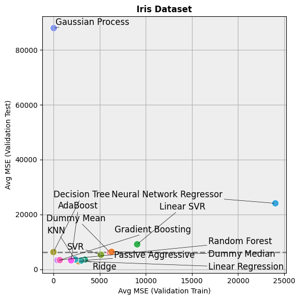
hh.plot_batch_results(df_results, metric_name="MSE", title="Iris Dataset", display=False)

# Take the models in positions 1, 2, 3 and 5
models = [i for _, i, _ in hh_models.trained_models[1:3] + hh_models.trained_models[4:5]]

# Plot the predictions
hh.plot_regression_pred(
    X,
    y,
    models=models,
    metric=mean_squared_error,
    title="Diabetes",
    y_label="Diabetes (Value)",
)

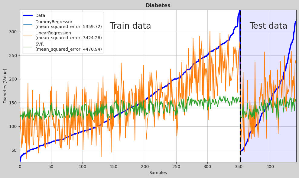
In case we needed to use one of the trained models, we can take it from the trained_models attribute from the HundredHammersRegressor class. This value will consist on a list with tuples containing the name of the model and the trained model.

hh_models.trained_models

[('Dummy Mean', DummyRegressor(), {}),
 ('Dummy Median', DummyRegressor(strategy='median'), {}),
 ('Linear Regression', LinearRegression(), {}),
 ('Decision Tree', DecisionTreeRegressor(random_state=9), {}),
 ('SVR', SVR(), {}),
 ('Linear SVR', LinearSVR(random_state=9), {}),
 ('Ridge', Ridge(random_state=9), {}),
 ('Passive Aggressive', PassiveAggressiveRegressor(random_state=9), {}),
 ('KNN', KNeighborsRegressor(), {}),
 ('Neural Network Regressor', MLPRegressor(random_state=9), {}),
 ('Gaussian Process', GaussianProcessRegressor(random_state=9), {}),
 ('Random Forest', RandomForestRegressor(random_state=9), {}),
 ('AdaBoost', AdaBoostRegressor(random_state=9), {}),
 ('Gradient Boosting', GradientBoostingRegressor(random_state=9), {})]

Automatic optimization of hyperparameters

In case we want to choose the models we want to evaluate, we must indicate them to the HundredHammersRegressor class.

For this example, we will use four simple regression models.

models_to_check = [
    ("Dummy", DummyRegressor(), None),
    ("Ridge", Ridge(random_state=0), None),
    ("Decision Tree", DecisionTreeRegressor(random_state=0), None),
    ("KNN", KNeighborsRegressor(), None),
]

Each model has a name and an object that implements it. The third position in the tuple represents the user-specified grid of hyperparameters, however, we will let them be automatically generated.

This will only happen for already configured models, if you want automatic generation of hyperparameters for a model that is not already added, check the “example_add_model.ipynb” notebook.

We can now proceed passing these models to the HundredHammersRegressor class.

hh_models = hh.HundredHammersRegressor(models=models_to_check, show_progress_bar=True)

This time, since we want to optimize the hyperparameters of our models, we set the appropriate parameter to True.

We can configure how many parameters to check in the GridSearch step, n_grid_points will indicate how many values each of the hyperparameters will take. In this case, we will take 8 values for each one. In the case of categorical values, if there are less than 8 values, only those will be taken.

df_results = hh_models.evaluate(X, y, optim_hyper=True, n_grid_points=8)

Evaluating models...: 100%|██████████| 4/4 [00:01<00:00,  3.37it/s]

df_results

	Model	Avg R2 (Validation Train)	Std R2 (Validation Train)	Avg R2 (Validation Test)	Std R2 (Validation Test)	Avg R2 (Train)	Std R2 (Train)	Avg R2 (Test)	Std R2 (Test)	Avg MSE (Validation Train)	...	Avg MSE (Test)	Std MSE (Test)	Avg MAE (Validation Train)	Std MAE (Validation Train)	Avg MAE (Validation Test)	Std MAE (Validation Test)	Avg MAE (Train)	Std MAE (Train)	Avg MAE (Test)	Std MAE (Test)
0	Dummy	0.000000	0.000000	-0.023206	0.033628	0.000000	0.000000e+00	-0.001337	0.000000e+00	6125.118931	...	5134.783503	0.000000e+00	67.301695	1.188564	67.615074	3.943941	67.339534	1.421085e-14	59.227456	7.105427e-15
1	Ridge	0.553573	0.015243	0.516564	0.064871	0.551601	1.110223e-16	0.333235	0.000000e+00	2733.434135	...	3419.120423	0.000000e+00	42.664323	0.836894	43.975160	3.176279	42.767356	0.000000e+00	46.036471	0.000000e+00
2	Decision Tree	0.705049	0.025423	0.227255	0.138329	0.663131	2.495672e-03	-0.061039	1.694207e-02	1806.214920	...	5440.928933	8.687768e+01	29.342648	1.290889	52.845684	4.971056	31.059490	3.552714e-15	57.152247	7.021638e-01
3	KNN	0.465824	0.017405	0.436415	0.061569	0.485286	5.551115e-17	0.315831	5.551115e-17	3270.483891	...	3508.367072	4.547474e-13	48.434238	0.888525	49.248325	2.949155	47.282775	0.000000e+00	47.117041	7.105427e-15

4 rows × 25 columns

Now that we have optimized the hyperparameters of the models, we can check which hyperparameters were chosen for each. This is done by checking the best_params attribute.

hh_models.best_params

[('Dummy', {'strategy': 'mean'}),
 ('Ridge', {'alpha': 0.03727593720314938}),
 ('Decision Tree', {'criterion': 'absolute_error', 'max_depth': 5}),
 ('KNN', {'metric': 'cosine', 'n_neighbors': 72})]

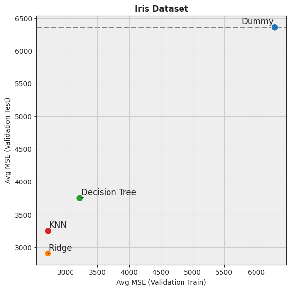
hh.plot_batch_results(df_results, metric_name="MSE", title="Iris Dataset", display=False)

Optimization of hyperparameters with custom parameter grids

For this example, we will use four simple classifier models with grids of hyperparameters.

These grid will contain all the paramaters that the gridsearch optimization will use.

models_to_check = [
    ("Dummy", DummyRegressor(), {"strategy": ["median"]}),
    ("Ridge", Ridge(random_state=0), {"alpha": [1e-4, 1e-3, 1e-2, 0.1, 1, 10]}),
    (
        "Decision Tree",
        DecisionTreeRegressor(random_state=0),
        {
            "criterion": ["squared_error", "absolute_error", "friedman_mse", "poisson"],
            "max_depth": [1, 2, 3, 4, 5, 6, 7],
        },
    ),
    (
        "KNN",
        KNeighborsRegressor(),
        {"n_neighbors": [1, 3, 5, 7, 9, 11], "metric": ["manhattan", "euclidean"]},
    ),
]

We can now proceed passing these models to the HundredHammersRegressor class.

hh_models = hh.HundredHammersRegressor(models=models_to_check, show_progress_bar=True)

Since we want to optimize the hyperparameters of our models, we set the appropriate parameter to True.

We don’t need to set the n_grid_points parameter since we have already chosen which parameters to take in the GridSearch step.

df_results = hh_models.evaluate(X, y, optim_hyper=True)

Evaluating models...: 100%|██████████| 4/4 [00:00<00:00,  6.63it/s]

df_results

	Model	Avg R2 (Validation Train)	Std R2 (Validation Train)	Avg R2 (Validation Test)	Std R2 (Validation Test)	Avg R2 (Train)	Std R2 (Train)	Avg R2 (Test)	Std R2 (Test)	Avg MSE (Validation Train)	...	Avg MSE (Test)	Std MSE (Test)	Avg MAE (Validation Train)	Std MAE (Validation Train)	Avg MAE (Validation Test)	Std MAE (Validation Test)	Avg MAE (Train)	Std MAE (Train)	Avg MAE (Test)	Std MAE (Test)
0	Dummy	-0.027476	0.007274	-0.050684	0.071611	-0.025922	0.000000e+00	-0.045202	0.0	6293.183322	...	5359.719101	9.094947e-13	66.517990	1.217067	66.993618	4.993507	66.566572	0.0	59.044944	0.000000e+00
1	Ridge	0.555347	0.015218	0.515900	0.066570	0.553033	1.110223e-16	0.329983	0.0	2722.561310	...	3435.796416	4.547474e-13	42.494128	0.829984	43.926355	3.180674	42.664912	0.0	46.170390	0.000000e+00
2	Decision Tree	0.473673	0.020150	0.373744	0.120035	0.477605	5.551115e-17	0.020330	0.0	3222.626891	...	5023.676966	0.000000e+00	43.848744	0.862175	47.866137	4.431692	44.014164	0.0	54.353933	7.105427e-15
3	KNN	0.554573	0.020198	0.459955	0.074056	0.548160	0.000000e+00	0.284378	0.0	2727.046694	...	3669.657350	9.094947e-13	41.663537	1.146837	45.521591	3.630353	41.737832	0.0	46.806946	0.000000e+00

4 rows × 25 columns

Now that we have optimized the hyperparameters of the models, we can check which hyperparameters were chosen for each. This is done by checking the best_params attribute.

hh_models.best_params

[('Dummy', {'strategy': 'median'}),
 ('Ridge', {'alpha': 0.01}),
 ('Decision Tree', {'criterion': 'absolute_error', 'max_depth': 2}),
 ('KNN', {'metric': 'euclidean', 'n_neighbors': 11})]

We can also show the plots like last time.

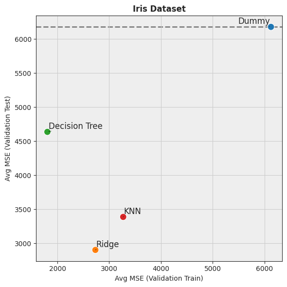
hh.plot_batch_results(df_results, metric_name="MSE", title="Iris Dataset", display=False)